Microsoft Excel is a popular software and is commonly used to perform data entry, accounting, financial analysis, etc. We can use it to make charts, graphs, and a little bit of programming.
It also organizes and presents data in meaningful categories. It is also used by businesses to keep records of sales, subordinates, and profits as well.
In this guide, we’ll be sharing the top 10 excel formulas that every working professional should know about.
What Is Microsoft Excel?
Microsoft Excel is a software that helps to organize, calculate and format data. It contains a spreadsheet system to process data that helps to record and analyze mathematical and statistical data.
Through MS Excel, anyone can easily present data in the form of charts and graphs. Charts and graphical representation can make the business presentation interesting and understandable.
How To Use Excel Formulas?
Excel is a powerful tool to perform mathematical and logical operations fast. It contains numerous formulas such as:
- SUM
- COUNT
- COUNTA
- COUNTBLANK
- AVERAGE
- MIN
- MAX
- LEN
- TRIM
- IF
1. SUM
SUM function is commonly used to find the sum of the value in two or more cells.
Example:
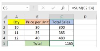
If you want to find the number of total sales, then you simply type “=SUM(C2:C4)” in the function bar. Now it will automatically provide the total value of sales.
2. AVERAGE
The AVERAGE function calculates the average of the selected range of cells.
Example:
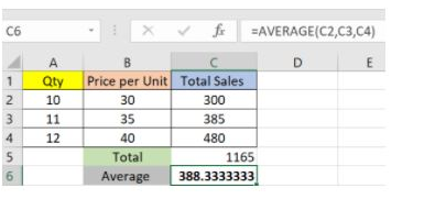
If you want to find the average of your total sales, then you just type “=AVERAGE(C2:C4)” in the function bar. Now it will automatically calculate the total average value of sales. You can easily fix this result in your desired location.
3. COUNT
The COUNT function counts the total number of cells with numerical values. This function does not count those cells containing text or other symbols.
Example:

To find the total number of cells in the total sales column, you just type “=COUNT(C1:C4)”.This formula will automatically present the total number of cells(3) in the Total Sales column.
If you want to find the total number of cells, including text and other symbols, then you use COUNTA( ) formula. For example, you simply type “=COUNTA( C1:C4)”. It will show 4 as an answer.
4. MAX
This basic function is used to find the maximum value from the selected range. In the below example, you can see the use of MAX( ).
Example:

You simply type “=MAX(A1:A5)” in the function bar and you will see the maximum number as a result.
5. SUBTOTAL
Do you know how the subtotal function works? You can easily calculate different values from the SUBTOTAL function, such as average, count and others. For it, you first write the base value in SUBTOTAL( ) and then select the range of data.
| Function | Base Value |
| Average | 1 |
| Count | 2 |
| Sum | 3 |
| Max | 4 |
| Min | 5 |
Example:
If you want to find the average of the Qty then you just write “= SUBTOTAL(1, A2:A4)” on the function bar. Then you will automatically find the average of Qty which is 11.
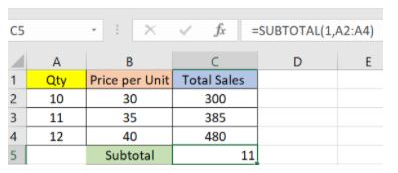
On the other hand, if you want to find the maximum value of Qty, then you simply type “=SUBTOTAL(4, A2:A4)”. Then it will easily provide the maximum numerical value of Qty which is 12.

6. MODULES
This function is helpful to find reminders. To find a reminder you just put dividend and divisor on this formula like “=MOD(dividend, divisor)”. In the below example you can see the function of MOD( ).
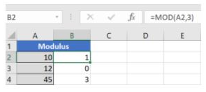
If you want to find a reminder of 10/3 then you simply type function bar MOD(A2,3). It will show you 1 as a reminder of this operation.
7. POWER
Through this function of excel you can easily find the power of any value. In the below example, you will see all the working of the POWER function.
Example:
If you want to find the cube root of the A2 cell, you just type POWER(A2,3) in the function bar. Then you will find the cube root of the A2 cell which is 1000. You can also use this function in the complete column by typing “=POWER(A,3)” in the function bar.

8. CELLING
It helps to round the decimal numbers into their nearest highest multiple. In the diagram below you will see this function how 35.316 turns into 40.
Example:

To apply this formula you simply write “=CELLING(A2,5)” in the function bar. It will provide you with 40 as the nearest highest value.
9. FLOOR
The FLOOR function helps to round a number down to the nearest multiple of significance.
Example:
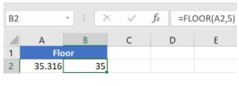
In the above diagram, you can see after applying the FLOOR formula on A2, it will turn 35.316 into 35.
10. LEN
This function is used to calculate the number of characters in a cell or text.
Example:
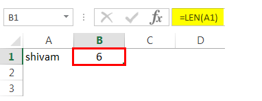
If you want to know about the number of characters in “Shivam” then you simply type “=LAN(A1)” in the function bar and you will find 6 as an answer.
Conclusion
Microsoft Excel is a very popular and vastly used platform throughout the world. It can perform mathematical and logical operations easily. In addition, it helps to present sales-related data as well as purchase-related data systematically.
It contains a spreadsheet that helps to perform mathematical operations such as addition, subtraction, multiplications, and dividend. You can perform many other logical operations, such as the AND function, IF function, and NOT function.


